Haozhe Zhang | HSTU 详解，以及把时间编码换成 RoPE / HSTU explained, and swapping its time encoding for RoPE

中文

推荐系统（recommender system，就是帮你排出”接下来最可能想看/想买什么”的那套模型）这十年基本都是两段式：先 retrieval（召回，从上亿候选里粗筛出几百个），再 ranking（精排，给这几百个打分排序），每一段都得喂一大堆手工特征。2024 年 Meta 那篇 Actions Speak Louder than Words 干脆把这框架掀了——把一个用户的整段历史当成一串 token，召回和精排统统变成”猜下一个 token 是什么”，也就是 generative recommender（生成式推荐，把 LLM 那套自回归玩法搬到推荐上）。撑起这套打法的新模块就叫 HSTU（Hierarchical Sequential Transduction Unit），它要顶替的是标准 transformer 里的 attention（注意力，序列模型里让每个位置去”看”别的位置的那个标准件）。

这篇就两件事。先把 HSTU 这个模块拆开，说清楚它跟普通 attention 到底差在哪；再聊一个我们自己在短视频数据上折腾出来的小结果——把它输入端的时间编码换成 RoPE（rotary position embedding，旋转位置编码：用一组随位置旋转的 sin/cos，把”谁先谁后、隔多远”塞给模型），离线指标涨了大概 1.5%。

从”排序”到”生成”：sequential transduction

传统精排说白了是个静态问题：给你一个用户、一批候选，吐出分数就完事。HSTU 把它改写成了 sequential transduction（序列转换，输入一串、输出一串，逐位置对齐）。做法是把用户历史里的 item（看过的视频、买过的东西）和 action（对它的反馈，完播、点赞、打分这些）交错串成一条序列：

\[\Phi_0,\, a_0,\, \Phi_1,\, a_1,\, \dots,\, \Phi_{n-1},\, a_{n-1}\]

这里 $\Phi_i$ 是第 $i$ 个 item 的 embedding（把离散 id 压成一个稠密向量），$a_i$ 是对应的 action。这么一摆，精排就是在每个 item 后面猜它的 action $p(a_{i+1}\mid \Phi_0, a_0, \dots, \Phi_{i+1})$，召回就是猜下一个 item $p(\Phi_{i+1}\mid u_i)$。原来要两套模型、两套特征工程伺候的事，现在塌成了同一个自回归目标——”生成式”三个字就是这么来的。

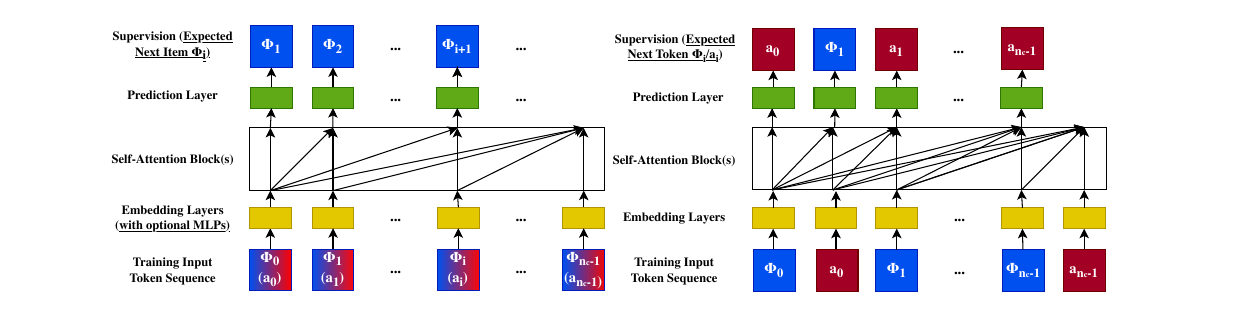
Traditional sequential recommender (left) vs generative recommender (right) (Fig. 8, Zhai et al. 2024): items and actions interleaved into one token sequence, predicting the next token.

这么搞最大的好处是 scaling：序列拉得越长、参数堆得越多，效果越好，跟 LLM 一个脾气。论文里 HSTU 一路怼到 1.5 万亿参数，公开 benchmark 上 NDCG（衡量排序质量的指标，越高越好）比基线高出一大截，线上 A/B +12.4%，推理还比 FlashAttention2 快 5–15 倍。

HSTU 这个 layer 内部长什么样

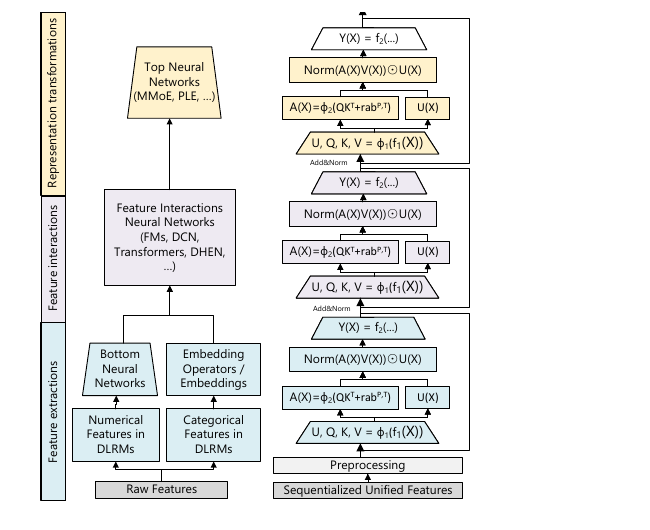
一个 HSTU layer 就三步。记输入的序列表征是 $X$。

第一步，pointwise projection（逐点投影）：一个线性层 $f_1(X)=W_1 X + b_1$ 一把算出四组向量，过一道 SiLU（$\phi_1$，一种平滑的激活函数）再切成四份：

\[U(X),\, V(X),\, Q(X),\, K(X) = \mathrm{Split}\big(\phi_1(f_1(X))\big)\]

$Q, K, V$ 就是 attention 里的老三样 query/key/value；多出来那个 $U$ 是个 gate（门控向量），留着第三步用。

第二步，pointwise aggregated attention（逐点聚合注意力）：

\[A(X)V(X) = \phi_2\big(Q(X)K(X)^\top + \mathrm{rab}^{p,t}\big)\,V(X)\]

注意这里的 $\phi_2$ 也是 SiLU，不是 softmax。这就是 HSTU 跟普通 transformer 最不一样的地方——attention 里那个”逐行归一化”的 softmax，被它直接换成了逐点的 SiLU。$\mathrm{rab}^{p,t}$ 是 relative attention bias（相对注意力偏置），把位置 $p$ 和时间 $t$ 当成一个加性偏置加到 $QK^\top$ 上，下一节再细说。

第三步，门控输出：

\[Y(X) = f_2\big(\mathrm{Norm}(A(X)V(X)) \odot U(X)\big)\]

把聚合结果归一化，跟第一步留下的 gate $U$ 逐元素一乘（$\odot$），再过个线性层。这套 gating 跟 GLU/SwiGLU 一个路子，让模型自己决定哪个通道放大、哪个压住。

$HSTU block vs a DLRM stack (Fig. 3, Zhai et al. 2024). Each HSTU layer: U,Q,K,V=phi1(f1(X)) -> A(X)=phi2(QK^T+rab^{p,t}) -> Norm(A(X)V(X)) (.) U(X) -> Y=f2(...).$

为什么要把 softmax 去掉

这步最反直觉，但也最关键。softmax 会把一行 attention 分数归一化成”加起来等于 1”的概率分布——它只留下相对大小，把绝对强度抹平了。可推荐里，”有多少条历史都指向同一个目标”恰恰是个极强的信号：一个人连刷 20 个篮球视频，跟只看过 1 个，你对”下一个该不该推篮球”的把握完全是两回事。softmax 一归一化，这种强弱差异就没了。HSTU 拿逐点 SiLU 换掉 softmax，图的就是把这个幅度/强度信息留住。论文原话大意是：指向目标的历史数据点数量，是用户偏好强度的强特征，而它在 softmax 归一化之后很难保下来。

代价是 attention 不再是概率分布、每行加起来也不为 1，所以才得靠第三步那个 Norm 加 gating 把数值范围拉回来。

HSTU 怎么编码位置和时间

序列模型自己不知道”谁先谁后”，得显式喂进去。HSTU 把这事放进 $\mathrm{rab}^{p,t}$ 里——一个同时带位置项（排第几）和时间项（两个真实时间戳隔了多久）的相对偏置，加在 $QK^\top$ 上。时间项尤其要紧，因为推荐数据是条非平稳的流：同样是两次点击，隔 5 分钟和隔 3 个月完全是两码事，时间项就是让模型看见这个 gap。

不过在 Meta 开源的 generative-recommenders 里，输入端那个 preprocessor（预处理模块，把 id 序列变成喂进 layer 的 embedding）默认用的其实是个可学习的绝对位置 embedding：把 item 和 action 交错成 $2N$ 长的序列，再按位置 index 查一张可学习的位置表加上去。时间信息主要还是靠 attention 里头 $\mathrm{rab}$ 那一项扛着。我们动的，就是输入端这块位置/时间编码。

我们的实验：把时间编码换成 rotary 时间戳编码

背景是我们一个小项目 HummingbirdRec，把 HSTU 搬到 KuaiRec（快手放出来的短视频公开数据集，带视频时长、完播率这些字段）上，跟 SASRec（一个很经典的 self-attention 推荐基线）对。在这个 setting 里我们试了件事：把输入端那个纯”可学习绝对位置 embedding”，换成带 rotary 时间戳编码的版本。

具体就是：从每条交互的 timestamp 里抠出 hour-of-day（这条交互发生在一天的第几个小时，0–23），用一组 RoPE 风格的 sin/cos 编码成向量，加到输入 embedding 上：

\[\theta_i = 10000^{-2i/d},\qquad \mathrm{enc}(h) = \big[\,\sin(h\,\theta_i)\,\Vert\,\cos(h\,\theta_i)\,\big]\]

$h$ 是这条交互发生的小时，$d$ 是 embedding 维度。代码大概长这样：

def apply_rotary_embedding(self, timestamps, dim):
    half_dim = dim // 2
    theta = 10000 ** (-2 * torch.arange(half_dim) / dim)
    embeddings = timestamps.unsqueeze(-1) * theta
    return torch.cat([torch.sin(embeddings), torch.cos(embeddings)], dim=-1)

# forward 里：从每条交互的 timestamp 取 hour-of-day，加到输入上
hour = [[datetime.utcfromtimestamp(ts).hour for ts in row] for row in timestamps]
user_embeddings = user_embeddings + self.apply_rotary_embedding(hour, dim)

换上之后，KuaiRec 上的离线 ranking 指标涨了大概 1.5%。算不上惊天动地，但方向稳，还几乎不要钱——没加参数，计算也没多多少。

为啥有用，有个挺朴素的解释：短视频消费的昼夜节律特别强。同一个人，通勤路上刷的、午休刷的、半夜躺床上刷的，口味根本不一样。把 hour-of-day 显式编进去，等于白送模型一个跟”什么时候在刷”对齐的特征。至于为什么用 sin/cos 而不是直接塞个整数小时——因为 sin/cos 天然把 23 点和 0 点放得很近（它是周期的），不会把这俩当成相差 23 的两个极端。

几个得说在前头的 caveat

严格讲，这版并不是经典 RoPE。经典 RoPE 是按位置去旋转 Q/K 向量、让相对位置体现在点积里；我们这儿是把时间戳的 sin/cos 编码直接加在输入 embedding 上，更接近 Transformer 原版那个 sinusoidal positional encoding，只不过喂进去的是时间戳、不是位置 index。叫它”rotary 时间戳编码”更老实。
只编了 hour-of-day，把 day-of-week、距上次多久这些一样有用的尺度全扔了。多尺度时间特征（小时 / 星期 / 距上次交互多久）估计还能再抠出一点。
1.5% 是个单一离线结果：就 KuaiRec 一个数据集、一套超参跑出来的，没上线、也没做多 seed 的显著性检验。当成”值得接着挖的信号”就行，别当结论。
它跟 HSTU 内部 $\mathrm{rab}$ 的时间项是叠加，不是替换——我们改的是输入端 preprocessor，attention 里那项还在。这俩怎么分工、会不会冗余，还没拆开测过。

接下来想做的

把 hour-of-day 扩成多尺度时间编码；把时间真正做进 attention（比如按时间戳去旋转 Q/K，而不是只在输入端相加）；以及在 KuaiRec 之外的数据集上把这 1.5% 复现出来，确认它不是单一数据集的运气。

English

For about a decade the standard recommender system (the thing that decides “what you’ll probably want next”) has been a two-stage pipeline: retrieval (pull a few hundred candidates out of hundreds of millions), then ranking (score and sort those few hundred) — each stage fed a big pile of hand-crafted features. Meta’s 2024 paper Actions Speak Louder than Words threw that framing out: treat a user’s whole history as a stream of tokens, and make both retrieval and ranking just “predict the next token.” That’s a generative recommender — the LLM autoregressive recipe, pointed at recommendation. The new block holding it together is HSTU (Hierarchical Sequential Transduction Unit), and what it’s replacing is the attention in a standard transformer (the part that lets each position in a sequence “look at” the others).

Two things in this post. First I’ll pull HSTU apart and show where it actually differs from ordinary attention. Then a small result we got on short-video data — swapping the input-side time encoding for RoPE (rotary position embedding: position-dependent sin/cos rotations that tell the model “what came before what, and how far apart”), which nudged our offline metric up by about 1.5%.

From “ranking” to “generating”: sequential transduction

Classic ranking is really a static problem: hand it a user and a batch of candidates, get scores back. HSTU rewrites it as sequential transduction (sequence in, sequence out, aligned position by position). You interleave the items a user touched (videos watched, things bought) with the actions taken on them (completion, like, rating) into one sequence:

\[\Phi_0,\, a_0,\, \Phi_1,\, a_1,\, \dots,\, \Phi_{n-1},\, a_{n-1}\]

where $\Phi_i$ is the embedding of item $i$ (a discrete id squeezed into a dense vector) and $a_i$ is its action. Laid out this way, ranking is just guessing the action after each item, $p(a_{i+1}\mid \Phi_0, a_0, \dots, \Phi_{i+1})$, and retrieval is guessing the next item, $p(\Phi_{i+1}\mid u_i)$. Two jobs that used to need two models and two feature pipelines collapse into one autoregressive objective — and that’s all “generative” means here.

Traditional sequential recommender (left) vs generative recommender (right) (Fig. 8, Zhai et al. 2024): items and actions interleaved into one token sequence, predicting the next token.

The big win is scaling: longer sequences and more parameters keep paying off, same temperament as LLMs. The paper pushes HSTU all the way to 1.5 trillion parameters, reports a large relative lift in NDCG (a ranking-quality metric, higher is better) over baselines on public benchmarks, +12.4% in online A/B tests, and 5–15× faster inference than FlashAttention2.

What a HSTU layer actually looks like

A HSTU layer is just three steps. Call the input representation $X$.

Step 1, pointwise projection. One linear layer $f_1(X)=W_1 X + b_1$ spits out four vectors at once; run a SiLU ($\phi_1$, a smooth activation) and split into four:

\[U(X),\, V(X),\, Q(X),\, K(X) = \mathrm{Split}\big(\phi_1(f_1(X))\big)\]

$Q, K, V$ are the usual query/key/value; the extra $U$ is a gate, saved for step 3.

Step 2, pointwise aggregated attention:

\[A(X)V(X) = \phi_2\big(Q(X)K(X)^\top + \mathrm{rab}^{p,t}\big)\,V(X)\]

Note that $\phi_2$ is also SiLU, not softmax. This is where HSTU parts ways with a normal transformer — the row-wise normalizing softmax in attention gets swapped for a pointwise SiLU. $\mathrm{rab}^{p,t}$ is a relative attention bias that drops positional ($p$) and temporal ($t$) info onto $QK^\top$ as an additive term (next section).

Step 3, gated output:

\[Y(X) = f_2\big(\mathrm{Norm}(A(X)V(X)) \odot U(X)\big)\]

Normalize the aggregate, multiply it element-wise ($\odot$) by the gate $U$ from step 1, run a final linear layer. The gating is GLU/SwiGLU-flavored — it lets the model decide for itself which channels to turn up and which to clamp.

$HSTU block vs a DLRM stack (Fig. 3, Zhai et al. 2024). Each HSTU layer: U,Q,K,V=phi1(f1(X)) -> A(X)=phi2(QK^T+rab^{p,t}) -> Norm(A(X)V(X)) (.) U(X) -> Y=f2(...).$

Why drop the softmax

This is the least intuitive part and the most important. Softmax squashes a row of attention scores into a probability distribution that sums to 1 — it keeps the relative sizes and flattens the absolute magnitude. But in recommendation, how many prior actions point at the same target is itself a strong signal: someone who just watched 20 basketball clips in a row is a completely different bet for “recommend basketball next” than someone who watched one. Normalize with softmax and that intensity is gone. HSTU swaps in a pointwise SiLU precisely to keep it. The paper’s own words, roughly: the number of prior data points related to the target is a strong feature for the intensity of user preference, and it’s hard to preserve after softmax normalization.

The cost: attention is no longer a probability distribution — rows don’t sum to 1 — which is exactly why step 3 needs the Norm and gating to pull the numbers back into range.

How HSTU encodes position and time

A sequence model doesn’t know “what came first” on its own; you have to feed that in. HSTU puts it in $\mathrm{rab}^{p,t}$ — a relative bias carrying both a positional term (which slot) and a temporal term (how much real time elapsed between timestamps), added onto $QK^\top$. The temporal term matters because recommendation data is a non-stationary stream: two clicks five minutes apart are a different animal from two clicks three months apart, and the temporal term is what lets the model see that gap.

In Meta’s open-source generative-recommenders codebase, though, the input-side preprocessor (the module that turns an id sequence into the embeddings fed to the layer) actually defaults to a learnable absolute positional embedding: interleave items and actions into a length-$2N$ sequence, then look up a learnable position table by index and add it. Time mostly rides on the $\mathrm{rab}$ term inside attention. What we changed is this input-side encoding.

Our experiment: swapping in a rotary timestamp encoding

The setting is a small project of ours, HummingbirdRec, which ports HSTU onto KuaiRec (Kuaishou’s public short-video dataset, with fields like video duration and watch ratio) and pits it against SASRec (a classic self-attention recommender baseline). In that setup we tried one thing: replacing the plain “learnable absolute positional embedding” at the input with a version that adds a rotary timestamp encoding.

Concretely: pull the hour-of-day (0–23) out of each interaction’s timestamp, encode it with a RoPE-style set of sin/cos, and add it to the input embedding:

\[\theta_i = 10000^{-2i/d},\qquad \mathrm{enc}(h) = \big[\,\sin(h\,\theta_i)\,\Vert\,\cos(h\,\theta_i)\,\big]\]

where $h$ is the hour the interaction happened and $d$ the embedding dimension. The code:

def apply_rotary_embedding(self, timestamps, dim):
    half_dim = dim // 2
    theta = 10000 ** (-2 * torch.arange(half_dim) / dim)
    embeddings = timestamps.unsqueeze(-1) * theta
    return torch.cat([torch.sin(embeddings), torch.cos(embeddings)], dim=-1)

# in forward(): pull hour-of-day from each interaction's timestamp, add it in
hour = [[datetime.utcfromtimestamp(ts).hour for ts in row] for row in timestamps]
user_embeddings = user_embeddings + self.apply_rotary_embedding(hour, dim)

With this in, the offline ranking metric on KuaiRec went up by about 1.5%. Not earth-shattering, but a stable direction and basically free — no extra parameters, negligible extra compute.

There’s a plain intuition for why: short-video consumption has a strong daily rhythm. What the same person scrolls on a commute, at lunch, and in bed at midnight just isn’t the same. Encoding hour-of-day explicitly hands the model a free feature lined up with when the scrolling happens. And the reason for sin/cos over a raw integer hour: sin/cos naturally puts 11pm and midnight right next to each other (it’s periodic) instead of treating them as two extremes 23 apart.

A few caveats worth stating up front

Strictly, this version isn’t classic RoPE. Classic RoPE rotates the Q/K vectors by position so relative position shows up in the dot product; what we did is add a sin/cos encoding of the timestamp to the input embedding, which is closer to the original Transformer’s sinusoidal positional encoding — just fed timestamps instead of position indices. “Rotary timestamp encoding” is the honest name.
It encodes only hour-of-day and throws away day-of-week and absolute inter-event gaps, which are useful scales too. Multi-scale time features (hour / weekday / time-since-last-interaction) would probably squeeze out a bit more.
The 1.5% is a single offline result — one dataset (KuaiRec), one hyperparameter setting, no online test, no multi-seed significance check. Treat it as a signal worth chasing, not a verdict.
It stacks on top of HSTU’s internal $\mathrm{rab}$ temporal term rather than replacing it — we touched the input-side preprocessor; the attention term is still there. How the two split the work, and whether they’re redundant, is untested.

What I’d do next

Grow hour-of-day into a multi-scale time encoding; push time properly into the attention (rotate Q/K by timestamp instead of only adding at the input); and reproduce the 1.5% on datasets beyond KuaiRec to make sure it isn’t single-dataset luck.